Machine Learning

Machine learning (ML) has broad applications in developing predictive models, including techniques such as linear regression, classification, and convolutional neural networks. Here shows an example from the Advanced Machine Learning Algorithms course by Stanford DeepLearning.AI, which I completed. This example is particularly suitable because it can be easily implemented using TensorFlow.

In astronomy, machine learning is typically applied to image data, with Convolutional Neural Networks (CNNs) being the primary model used due to their success in computer vision tasks. One notable example is ClaRAN (Wu et al. 2018), a deep learning classifier for radio morphologies developed by my colleague. I utilized this pre-trained CNN in my own project on dwarf galaxies and may eventually share the code on my GitHub page.

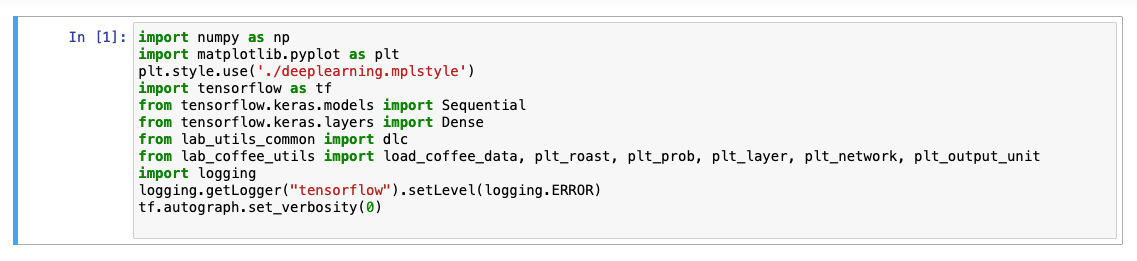
Step 1

Importing the required libraries and packages, and loading the dataset.

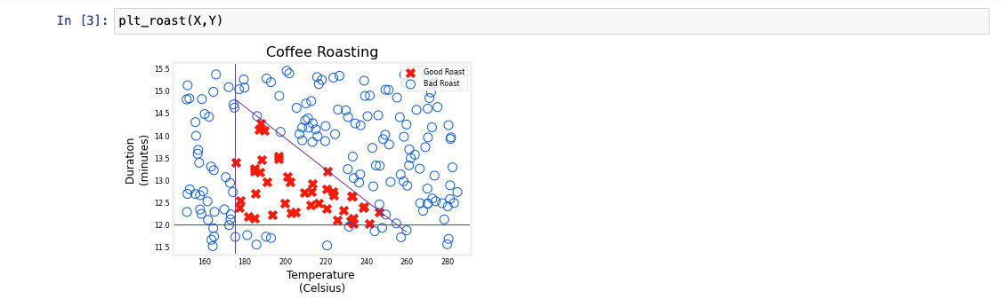
Step 2

Plotting the roasting data - Temperature vs Duration. The function of plt_roast is another Python script, which is not shown here. The recommended roast parameters are provided by the roasting company.

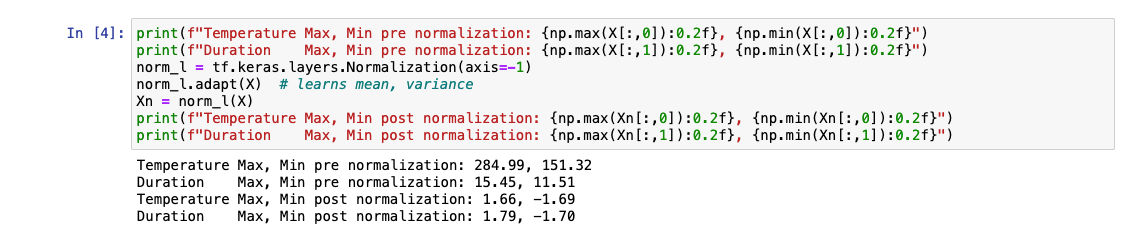
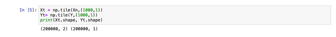
Step 3

Performing nomalization. "Regularization" is necessary when the data samples vary widely in range. Also, I experimented with increasing the training data set size and reducing the number of training cycles.

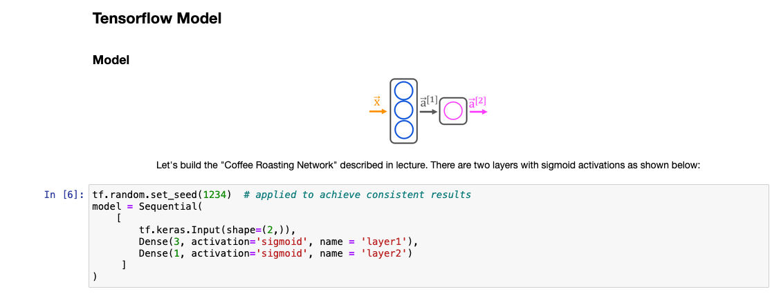
Step 4

Building the neural network - two layers. I utilized TensorFlow, which Sigmoid function is commonly used as an activation function.

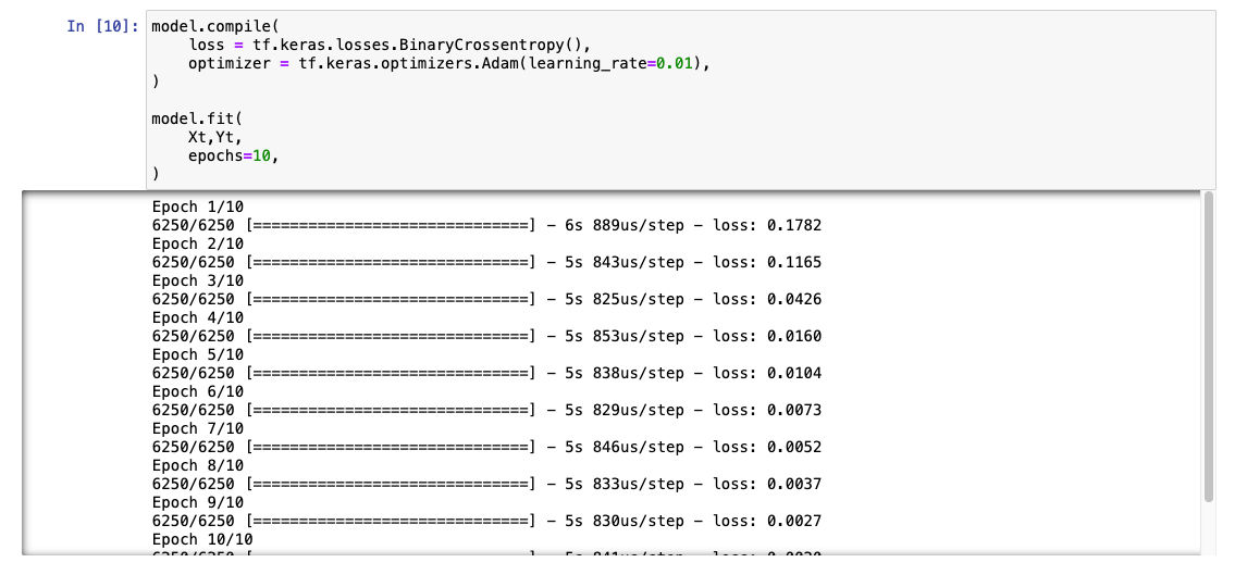
Step 5

Compiling the model and performing the fit.

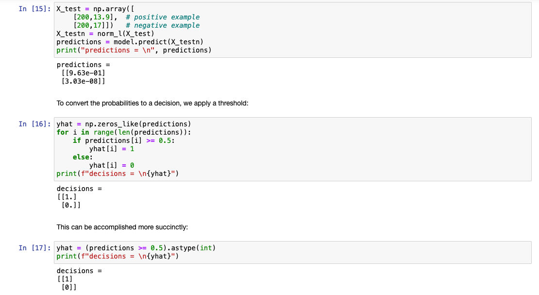
Step 6

Experimenting with different weights (not shown here), generating the predictions and converting the probabilites to a decision (1 or 0 from the Sigmoid function.

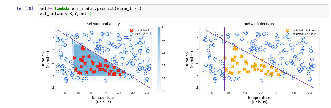
Step 7

The final outputs from model along with visualizations. The plt_network function is another Python script that is used to generate the plot (not shown here). Left: The blue shading represents the raw output from the final layer of the network. Right: The corresponding classification decisions made by the model.